→ Go to Part 3 (Advanced) [TBD]

Part 2: Reverse-mode autodiff

In part 2, we introduce AD tools for vector-matrix computations, and a more powerful reverse-mode technique especially useful in machine learning.

A brief recap of Part 1

In part one, we introduced the basics ideas of autodiff. In particular, we saw how forward-mode autodiff allows us to compute derivatives of any scalar function with a small, constant overhead.

To recap visually:

The colored instructions are those that we need to add to our original program (the primal program) to automatically include computation of a derivative.

If derivatives can be computed with a similar overhead to the original instructions (step 2, in blue), then it is easy to understand that this has (roughly) twice computational complexity as the original program.

Moving onwards: vector operations

To understand the limitations of the forward-mode technique, we make a step towards more realistic implementations, and we consider vector/matrix operations. We begin with a very small introduction to vector algebra: if you have no trouble with matrix computations, feel free to skim a few paragraphs to the next section.

Remember that a vector $\mathbf{x}$ is simply an ordered collection of $n$ scalar values:

$\mathbf{x} = \begin{bmatrix} x_1 \\ \vdots \\ x_n \end{bmatrix} \,.$

(We use bold to denote vectors, and $x_i$ to denote the element in position $i$ of the vector $\mathbf{x}$ .)

A vector-valued function is like a classical function, but it takes a vector $\mathbf{x}$ in input, and returns us with a vector $\mathbf{y}$ in output:

$\mathbf{y} = f(\mathbf{x}) \,.$

An example of a vector operation is a simple matrix multiplication:

$\mathbf{y} = \mathbf{W}\mathbf{x} \,.$

Vectors, matrices, and other higher-dimensional tensors are in fact the basic type in NumPy, JAX, or any deep learning library. The reason is that matrix computations enjoy very fast, optimized code for their execution. Because JAX follows the NumPy interface, we can write the above as:

def mvm(x, W):
    return np.dot(W, x) # Or W @ x

where mvm stands for matrix-vector multiplication. In order to extend the forward-mode AD operations from part 1, we need two things:

A definition of derivatives for a vector operation (blue step above).
An extension of the chain rule for composing elementary vector-valued functions (green step above).

Combining the two should then give us a way to extend forward-mode AD to vectors.

Step 1: A primer in matrix calculus

Thinking of derivatives as perturbations of the output w.r.t. the input, you see that there are many such perturbations here: one for every element of the vector in input and every element of the vector in output. If $\mathbf{x}$ has $n$ elements and likewise $\mathbf{y}$ has $m$ elements, then we have $mn$ partial derivatives $\frac{\partial y_i}{\partial x_j}$ , that are computed in a similar way to classical derivatives.

We can also organize the derivatives into a $m \times n$ matix, that we call the Jacobian of the function (keep in mind the dimensions, they will come in handy shortly):

$\mathbf{J}_f = \overbrace{ \begin{bmatrix} \frac{\partial y_1}{\partial x_1} & \ldots & \frac{\partial y_1}{\partial x_n} \\ \vdots & \vdots & \vdots \\ \frac{\partial y_m}{\partial x_1} & \ldots & \frac{\partial y_m}{\partial x_n} \\ \end{bmatrix} }^{\text{One column: one input}} \Biggl.\Biggr\}{\scriptstyle\text{One row: one output}}$

One very important case is $m=1$ , i.e., functions with many inputs but a single output. Most machine learning applications are of this type, where the final output is a single scalar (the loss) to be minimized. In this case, the Jacobian is a row vector, and its transpose is called the gradient of $f$ , denoted as $\nabla f$ . Computing the gradient efficiently is the building block of (almost) every optimization routine, so it will be our foremost concern below.

Step 2: A chain rule for matrices

To proceed, we need differentiation rules. Just like we have automatic rules for scalar functions, we have similar rules for vector-valued functions. For example, for scalars, we have that the derivative of a multiplication is $\frac{d}{dx} ax = a$ . In analogy, for our earlier matrix multiplication mvm, we have:

$\mathbf{J}_{\text{mvm}} = \mathbf{W} \,.$

(If you reason on it, it makes a lot of sense: the perturbation of input $x_j$ on output $y_i$ is exactly quantified by the single element $W_{ij}$ .)

Time to go bigger! Let us compose many functions now:

def g(x, list_of_functions):
    z = x
    for f in list_of_functions:
        z = f(z)
    return z

In order to proceed, we need the equivalent of the chain rule for matrix operations. Luckily, it has a very simple extension to the matrix domain. Consider two functions $f_1$ and $f_2$ , operating on vectors, and their composition, that we denote as $f_2 \circ f_1$ . We first apply $f_1$ to get a new intermediate vector $\mathbf{z} = f_1(\mathbf{x})$ , then apply $f_2$ to obtain the final vector $f_2(\mathbf{z})$ .

$f_1$ will have its own Jacobian (with respect to $\mathbf{x}$ ) that we denote with $\mathbf{J}_{f_1}$ , while $f_2$ will have a second Jacobian (with respect to its argument $\mathbf{z}$ ), that we denote by $\mathbf{J}_{f_ {2}}$ . Unsurprisingly, the chain rule for vectors tells us that the final Jacobian is the product of the two:

$\mathbf{J}_{f_2 \circ f_1} = \mathbf{J}_{f_2} \mathbf{J}_{f_1} \,.$

We have now circled all the way back to part 1: in order to do forward-mode AD for vector-valued functions, augment every elementary operation with the computation of the left-most Jacobian above, and multiply this by the Jacobian from the previous instruction. The resulting program will compute the function and the Jacobian simultaneously. Let us sketch this idea in code:

def gprime(x, list_of_functions, list_of_jacobians):
    z = x
    J1 = 1.0 # Initial Jacobian
    for f, jac in zip(list_of_functions, list_of_jacobians):
        J2 = jac(z) # Compute the local Jacobian
        z = f(z) # 2: Apply the original function
        J1 = np.dot(J2, J1) # Chain rule for Jacobians
    return z, J1

This strategy works: in fact, we can do it automatically in JAX with jacfwd(g), obtaining a very similar result as gprime above. However, its elegance hides a very serious drawback.

Towards reverse-mode autodiff

Consider the composition of three matrix multiplications, where the last one returns a scalar:

$y = \mathbf{w}_3^T\mathbf{W}_2\mathbf{W}_1\mathbf{x} \,.$

(It looks like a basic neural network with no activation functions.)

We know the rule for computing the Jacobian of a matrix multiplication. By applying it, we get a simple formula:

$\mathbf{J} = \mathbf{w}_3^T\mathbf{W}_2\mathbf{W}_1 \,.$

Remember that, in gprime, we execute the instructions from right to left: can you spot the problem? Our original program only requires vector-matrix multiplication, while adding the AD component requires a series of matrix-matrix multiplications! It means that the AD part will be $n$ times slower (roughly) than the original part. Because machine learning application can have billions of inputs (the parameters of a model) and just one output, this is seriously problematic.

Looking at the equation above also gives us a solution: we can obtain the Jacobian using vector-matrix operations by running the multiplications… left-to-right! In order to do this, we need to:

Store all local Jacobians while we execute the code.
Apply the chain rule in reverse on them.

This is our second mode of autodiff: unsuprisingly, it is called reverse-mode autodiff. It requires a lot more memory than forward-mode (for reason 1 above), and it must run after the original program (not in an interleaved fashion), but it is generally more efficient when we have few outputs. This is implemented in JAX with jacrev.

Summarizing:

$\mathbf{J} = \underset{\xrightarrow{\color{red}{Reverse-mode \,\,(jacrev)}}}{\overset{\xleftarrow{\color{green}{Forward-mode \,\, (jacfwd)}}}{\mathbf{w}_3^T\mathbf{W}_2\mathbf{W}_1}} \,.$

Understanding forward-mode vs. reverse-mode

First of all, let us see reverse-mode in action on the same function we used in Part 1:

def f(x):
  for i in range(3):
    x = 4*x*(1 - x)
  return x

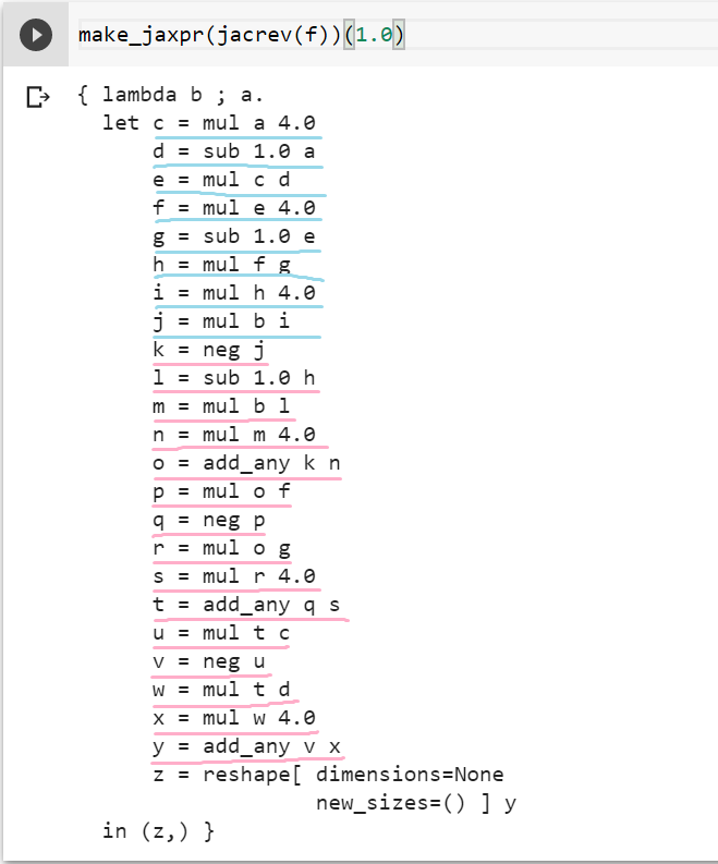
Just like in Part 1, we use blue for the original instructions, and red for the autodiff instruction. In this case, the original program is executed first, then a corresponding set of instructions (called the adjoint program) is executed to compute the partial derivatives. If you inspect it closer, you will see that for every variable, the sooner it is needed in the original program, the later it is needed in the adjoint.

In order to get more insights, consider reverse-mode autodiff applied on a function with many inputs and a single output. Every step of autodiff requires an operation of the form $\mathbf{v}^T\mathbf{J}$ , where $\mathbf{J}$ is the local Jacobian and $\mathbf{v}$ is the output of the previous iteration. If you go through the math, you will see that something similar is needed when you do forward-mode autodiff on a function with one input but many outputs. This brings us to our two final points.

Implementation of autodiff

First, we can understand on a sketch level how an autodiff mechanism, like in JAX, is implemented.

For every instruction in our code, autodiff requires the computation of the corresponding Jacobian-vector product (JVP) for forward-mode, or vector-Jacobian product (VJP) for the reverse-mode (in fact, only one is needed, and the other one can be obtained by tranposition)

If we know the JVPs of all primitives instructions in the library, we can autodiff almost automatically! Interestingly, specifying a JVP allows us to perform both forward-mode and reverse-mode.

If you want to experiment, autodidact is a small, didactic version of Autograd (a predecessor of JAX) to showcase the implementation of a minimal autodiff tool. For example, here is the definition of a small number of VJPs:

defvjp(anp.exp, lambda g, ans, x: ans * g)
defvjp(anp.log, lambda g, ans, x: g / x)

And of course, you can differentiate a lot more than pure mathematical functions. For example, here is the VJP for a reshaping operation:

defvjp(anp.reshape, lambda g, ans, x, shape, order=None:
       anp.reshape(g, anp.shape(x), order=order))

You can also inspect the full code of the reverse-mode operation. This set of slides gives some insights on the implementation of Autograd.

Finally, you can check this guide to understand how to implement new primitives in JAX.

Complexity of autodiff

What happens if we run reverse-mode autodiff with two outputs? For example, consider:

$\begin{bmatrix} y_1 \\ y_2 \end{bmatrix} = \begin{bmatrix}\mathbf{w}_{3,1}^T \\ \mathbf{w}_{3,2}^T \end{bmatrix}\mathbf{W}_2\mathbf{W}_1\mathbf{x} \,.$

If you check the equations, the answer is relatively simple: you need to run the entire process twice, starting from $\mathbf{w}_{3,1}$ and $\mathbf{w}_{3,2}$ .

Generalizing, we need (roughly) $m$ (where $m$ is the number of outputs) VJPs. In other words, we are computing the final Jacobian one row at a time, and every row requires more or less the same cost as the original program.

Similarly, for forward-mode autodiff, we need $n$ (where $n$ is the number of inputs) JVPs. In other words, we compute the final Jacobian one column at a time, and every column requires more or less the same cost as the original program.

For machine learning, where we have millions (or billions) of inputs and a single output (the loss) reverse-mode autodiff has of course become the standard. When reverse-mode autodiff is applied to a neural network, it is known more commonly as backpropagation. The drawback is that all intermediate results must now be stored: reverse-mode autodiff is memory hungry!

Conclusions

It tooks us a while, but we now have most basic instruments to understand autodiff. In the next parts, we will describe some interesting applications of both forward-mode and reverse-mode, as long as some interesting concepts from the theory of autodiff and its history.