Part 1: What is autodiff?

Remember: in this first part, we introduce what is, in fact, autodiff, and how to use it in JAX, by restricting our attention to scalar values and forward-mode autodiff. Have fun!

The limits of symbolic differentiation

First of all: why do we even care about how to compute derivatives? If you remember high-school calculus, you know that taking derivatives is a largely automatic process. You start from a symbolic expression, $f(x)$ , then apply a set of standard rules (e.g., the chain rule) to obtain its derivative, $f'(x)$ . Boring, maybe, but not too complex. Surely, something that a computer can do at ease.

Yet, symbolic differentation (as this process is called) is largely inefficient. In fact, nothing prevents an exponential increase in the complexity of $f'(x)$ . To demonstrate it, let me take this example from a survey paper¹ (which, coincidentally, should be your first technical reading if you really want to understand the theory behind all of this):

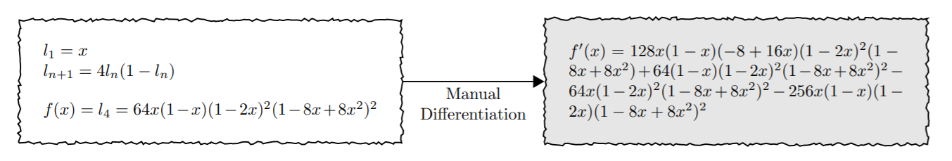Fig. 1: symbolic differentation, adapted from (Baydin et al., 2017).¹

If you inspect closely the symbolic expression for $f'(x)$ , on the right, you will see many repeated expressions (and some general ugliness, when compared to the elegant expression on the left). While we can try to simplify it, we do not have any guarantees on the size and complexity of the outcome. To proceed, we must find a smarter way.

From symbols to computer programs

In order to make some progress towards a more efficient solution, let us look at a possible implementation of the function:

def f(x):
  for i in range(3):
    x = 4*x*(1 - x)
  return x

In addition, we remember the chain rule of derivation: given a function $f(x)$ and another function $g(x)$ , the derivative of their composition is (ignoring colours for a moment):

$\frac{d\left[f(g(x))\right]}{dx} = \color{blue}{f'(} \color{red}{g(x)} \color{blue}{)} \cdot \color{green}{g'(x)} \,.$

The chain rule is the foundation of all autodiff systems, both for scalar functions (like here) and for vector-valued functions, covered in Part 2. It is instructive to look at it very closely, especially when considering its application to a computer program, where $f$ and $g$ are two instructions to be executed one after the other.

Let us assume to have already computed the first instruction $g(x)$ (the red part above), and its corresponding derivative $g'(x)$ (the green part above). Then, after applying $f$ , updating the derivative only requires the computation of $f'$ (the blue part above) and a simple multiplication.

If we combine the chain rule with our previous code, we thus get an equally concise code to compute the function and the derivative simultaneously:

def fprime(x, df=1.0):
  for i in range(3):
    x = 4*x*(1 - x)
    df = df * (4 - 8*x) # Chain rule!
  return x, df

The derivative is initalized to $1.0$ (because $\frac{dx}{dx}=1.0$ ). Then, after every update of $x$ , we do a corresponding update of the derivative with a straightforward application of the chain rule.

In case you were wondering: this is an example of autodiff! In particular, this is called forward-mode autodiff. Starting from an implementation of the function we want to differentiate, we augment every call inolving $x$ with a corresponding chain rule application to update the derivative. The result, unsurprinsingly, allows us to compute the derivative with only a constant (time and memory) overhead.

This is the first, key result: autodiff fundamentally works at the level of computer programs, while our high-school calculus mostly cared about the definition of the function. This picture from Wikipedia sums up the concept well:

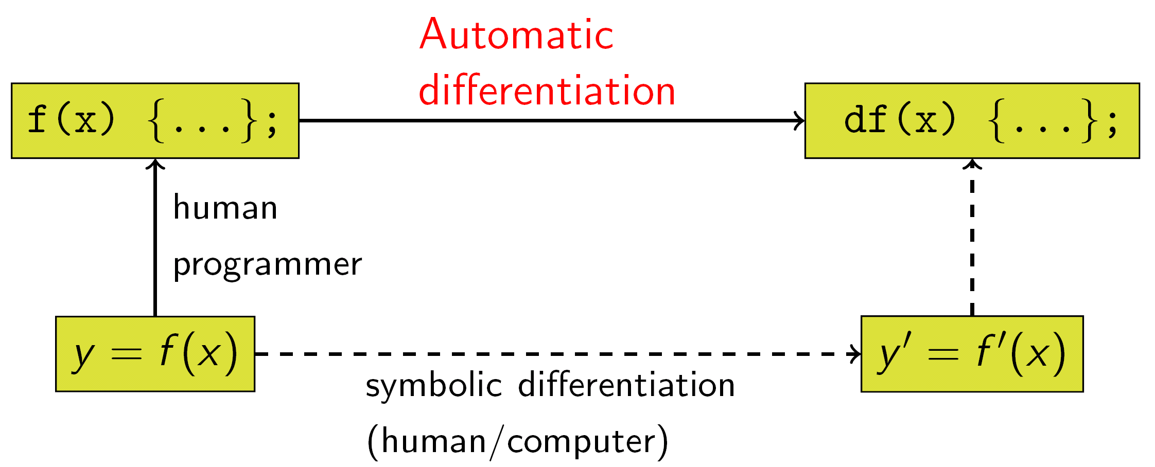Fig. 2: symbolic vs. automatic differentiation (from Wikipedia).

Automating the differentiation

Of course, the process we followed above can be automated. In fact, we can let JAX build the function for us:

from jax import jacfwd
fprime_jax = jacfwd(f, argnums=0)

jacfwd is the first important transformation from JAX that we introduce in these tutorials. It traces the execution of f, and returns us with an implementation of fprime that performs forward-mode AD for us.

In case you are wondering, the name jacfwd will become clear in the next part.

The only requirement for jacfwd, or any other JAX transformation, is that the function must contain only JAX instructions or instructions that JAX can understand, such as simple control flow routines (we will come back on this later on).

It is instructive to see what happens when we run this code on some concrete data. For this, we exploit another JAX transformation, make_jaxpr. The function allows us to trace the execution of any other JAX-compatible function, and returns us with a jaxpr, a tree of computations defined in an internal low-level language. Let us see a very simple example:

make_jaxpr(lambda x: np.sin(x) + 3.0)(1.0)

{ lambda ; a.

let b = sin a

c = add b 3.0

in (c,) }

While fully understanding the jaxpr syntax is long, the above example should be clear enough. The high-level Python code is translated to a series of low-level instructions. In fact, the expression works as a middle ground between the code we write, and the platform-specific implementation of the low-level instructions. In addition, it is the basic instrument that JAX uses to perform code transformations, of which jacfwd is our first example.

Let us inspect the jaxpr for our fprime_jax. I will manually highlight in red/blue the instructions corresponding to our original function and to the AD bits:

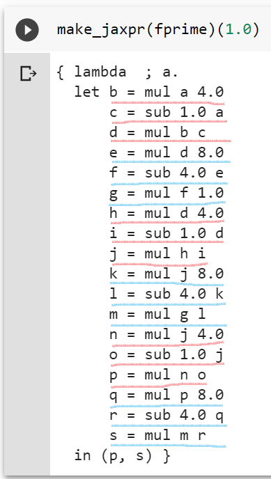
By this point, the complete symmetry of the code should not surprise you. For every instruction, forward-mode AD inserts a corresponding application of the chain rule. Because derivatives are generally very similar to the original function, we get something like above.

Are we done yet?

It looks like we are very close to a complete solution. We have seen a technique to obtain a derivative from any function, using only a small overhead in terms of time and space.

For the moment, we have focused on scalar values. We will see in the next part that, moving to vectors and matrices, things are more complex, and forward-mode AD has some serious limitations (particularly when applied to machine learning). For this reason, we will introduce a different version, reverse-mode autodiff, to overcome them. We will also start discussing the way AD systems can be implemented.

→ Go to Part 2 (Vectors)

Footnotes

Baydin, A.G., Pearlmutter, B.A., Radul, A.A. and Siskind, J.M., 2017. Automatic differentiation in machine learning: a survey. The Journal of Machine Learning Research, 18(1), pp.5595-5637. ↩ ↩²

The magic behind autodiff